The Economics of Static Analysis Tool Usage

The Model

Many factors contribute to the economics of static analysis tool use; and the relationships between them are not always straightforward. The model I introduce here is a coarse approximation that attempts to capture the important aspects of the process. It attempts to be useful while remaining simple, so some subtleties are not considered.

Let f(P) be the function that maps the precision of a tool to the probability that a true positive is recognized correctly. The effectiveness of a tool, i.e., the number of real defects found and recognized as such is thus given by:

N × R × f(P)

Where N is the number of defects found, R is the recall, the measure of the ability to find real defects, and P is the precision, the ability of the tool to exclude false positives. There is more background on these definitions in my previous post. Given these definitions, we can see how good some example tools are at finding real defects.

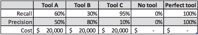
Let us now consider three hypothetical tools (or configurations of the same tool) that occupy a position along the recall-precision spectrum discussed earlier.

• Tool A is reasonably good at finding defects, with a recall of 60%. Half of the results it reports are false positives.
• Tool B has a precision of 80%, meaning it is very good at suppressing false positives. However, it finds only 30% of the real defects.
• Tool C has a recall of 95%, so is extremely good at finding defects, but its precision is only 10%.

It is also useful to consider two other cases: the mythological perfect tool that finds
all defects with no false positives, and not using a static analysis tool at all. The tool properties are summarized in Figure 1.

 

Figure 1: Properties of the example tools.

Let us suppose that the number of defects that are not detected by other means is N=100. Figure 2 shows the raw results from the tools.

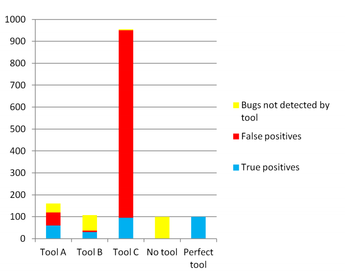
Figure 2: The raw results of the example tools

Now what really matters is how those raw results are interpreted. As discussed in my previous post, some real defects will not be recognized as such. Figure 3 shows two histograms of the defects that remain in the application under the linear and cubic models for true positive recognition.

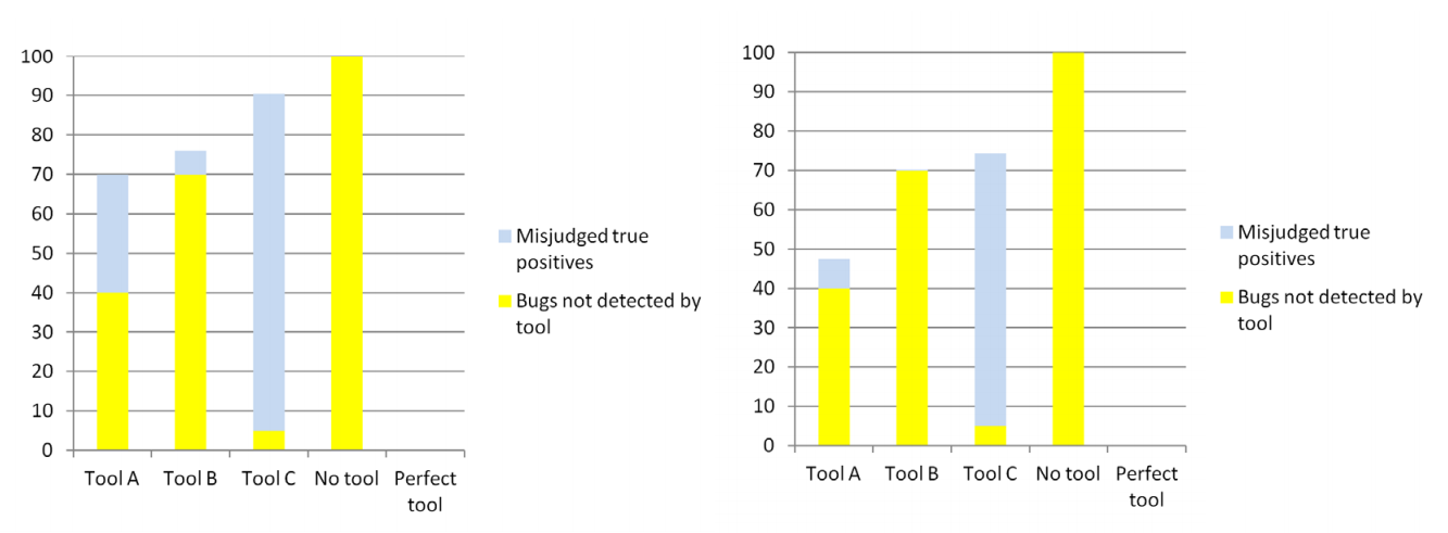
Figure 3: The number of defects that remain in the application for the linear (left) and cubic (right) true positive recognition models. Clearly, fewer defect totals are better.

What emerges from this model is that there is a sweet spot in the tradeoff between precision and recall. Tool A had worse precision than tool B and worse recall than tool C, but when it is used, fewer defects remain in the application.

Economics

Now we can model the economic aspects of the process. The important inputs are the following:

The probability and cost of an incident caused by a defect. Software defects and security vulnerabilities are depressingly commonplace, but not all of them cause serious problems. Many lie dormant and unexploited before they are removed through routine maintenance. This can be modeled by assigning a probability that a defect will trigger an incident during the lifetime of the product. If a defect does cause an incident, there will be a cost of dealing with that incident, and this cost can vary enormously. Incident consequences can include product recall, disruption to service, damage to reputation, theft of property, litigation, and even death or injury if the application is safety critical. The best case is that few customers are harmed or inconvenienced by the defect and that the defect is fixed and deployed through normal maintenance processes, but even that has a cost. The numbers shown below in Figure 4 are based on a probability of 5% and an example incident cost of $40,000.

The time to correct a defect. Regardless of whether a defect causes an incident, there is an engineering cost to fix it. Bugs that are found earlier are much less expensive to fix. Those that are found later can be especially costly to fix as the product may have to be retested. In the calculations below, we assume it takes 4 hours to fix a bug early in the development cycle, versus 20 to fix it after deployment. These numbers are based on a 2002 NIST report.

Figure 4: Cost breakdown for the example tools (left), and the benefit of using each tool compared to using no tool (right). These numbers are derived from the values discussed in the previous paragraphs.

Again the tool that strikes a reasonable balance between precision and recall is the one that is most beneficial to use. Tool A is more beneficial even though it found only about half as many real defects as Tool C, and had eight times more false positives than Tool B. It is also interesting to note that Tool C sits slightly below the break-even point, even though it has the highest recall.

The relative order of the tools is fairly insensitive to the actual numbers used for the cost and the probability of an incident as long as the cost of an incident exceeds the cost fixing the defects found by the tool. In such an extreme case however, the most cost-effective strategy is to use no tool at all.

This model confirms that the benefit of using a static analysis tool is dominated by its ability to find real defects that are subsequently recognized as such. Although there is a cost to triaging the warnings, this is relatively minor compared to the cost of an incident. Consequently, we can conclude that a tool’s effectiveness, i.e. its ability to find real defects that are correctly recognized as such, is a good approximation to its overall benefit. Note however that this requires knowing the value of recall, which as discussed earlier is notoriously elusive. The next section describes how we can eliminate that unknown and use the model to compare tools using easily harvested data. 

Users generally feel better about configurations that keep false positives very low, but the model shown here demonstrates that the sweet spot that maximizes the benefit of using the tool means it is worth tolerating a much higher false positive rate as long as the tool is also finding more real issues.